Blank

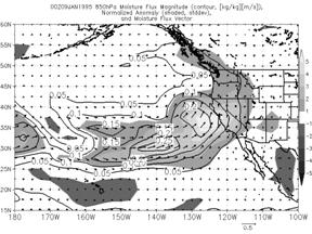
850-hPa moisture flux (arrows) and magnitude of the moisture flux (solid) and anomaly of the magnitude of the moisture flux (shaded, unit= 1SD) valid 0000 UTC 9 Jan 1995.

5 SD

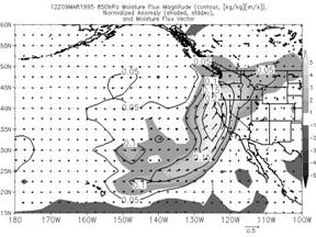
850-hPa moisture flux (arrows) and magnitude of the moisture flux (solid) and anomaly of the magnitude of the moisture flux (shaded, unit= 1SD) valid 1200 UTC 9 Mar 1995.

All three events were associated with plumes of moisture that impinged upon the coast. The role of these plumes or atmospheric rivers is even more evident when anomalies of the magnitude of 850-hPa moisture flux is examined. Let’s first look at the moisture flux anomalies associated with the January and March 1995 events (see below). The shaded areas are anomalously high MF anomalies with the white area having a 5 SD departure from normal.

The 5 SD moisture flux anomaly impinging upon the coast suggests that the both 1995 rainfall events might be relatively rare as more than 99.999% of the time the moisture flux will be lower than on the two maps above. Significant flooding and flash flooding also occurred over the Sacramento, Napa, and Sonoma Valleys as a result of rainfall during the eight-day period, January 7-15, 1995 (NOAA 1995), prompting thirty-four counties to be declared federal disaster areas. The March 9-10, 1995 caused considerable flooding on the San Joaquin basin (Reynolds 1996). The combined damage from the January and March 1995 floods exceeded 305 million dollars in the Sacramento Valley and 193 million in the San Joaquin Valley (Army Corps of Engineers 1999).

Let’s explore the 850-hPa moisture flux and MF anomalies during the period from 0000 31 Dec. 1996 through 0000 UTC 2 Jan. 1997 and explore the relationship of the maximum rainfall to the axis of strongest 850-hPa MF. During the entire period, the standardized MF anomalies were at least 4 SD and usually 5 SD. Again the normalized anomaly pattern signalized that there was the potential for a relatively rare, extreme rare precipitation event over California. This particular event, caused nearly two billion dollars in property damage and forced over 100,000 people from their homes (Baird and Robles 1997).

850-hPa moisture flux (arrow, scale shown at bottom of image), magnitude of moisture flux (interval=0.05 ms^-1) and normalized anomaly of moisture flux (magnitude of the anomaly is shaded with the scale on the right hand side of the figure, interval=1 SD) for a) 0000 UTC 31 Dec. 1996, b) 1200 UTC 31 Dec. 1996, c) 0000 UTC 1 Jan. 1997, and d) 0000 UTC 2 Jan. 1997.

During upslope events, the anomalously moisture flux impinging upon the coast and mountains helps determine the location of where the heaviest rainfall will occur. The axis of strongest moisture flux was located north of San Francisco during the 24 hour periods ending at 1200 UTC 31 Dec. 1996 and 1200 UTC 01 Jan. 1997. By 0000 UTC 2 Jan. 1997 the axis had shifted south of San Francisco, only then did very heaviest rainfall shift south of the city (see figures below).

24 hr HPC precipitation analysis for, a) 1200 UTC 31 Dec 1996, b) 1200 UTC 1 Jan 1997, and c) 1200 UTC 2 Jan 1997. From Junker et al. 2007

All three of these multi-day rainfall events was associated with a “pineapple express” or atmospheric river where there was anomalously high PW and MF. Ralph et al. (2006) seven floods on the Russian River that were associated with landfalling atmospheric rivers attesting to their importance in producing excessive rainfall.

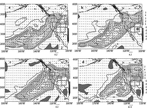
Composite mean standardized 850-hPa moisture flux anomalies of moisture flux field at the beginning of the period of heavy rainfall, a) for 4 inch or greater events and b) for 2-4 inch events; at the end of the period, c) for 4 inch or greater events, and d) for 2-4 inch events (from Junker et al. 2007).

There are differences in the moisture flux and PW anomaly fields between events that produce heavy rainfall compared to those that produce more modest amounts (see above). Note that 500-hPa departures from normal indicate that the shortwaves associated with the heaviest events are slower moving than the more moderate ones. The differences in the anomaly fields for moderate and heavy support the idea that anomalies can be used to identify major rainfall events. The similarity of the 500-hPa, 700-hPa and 850-hPa moisture flux patterns at locations from the Pacific Northwest (Lackmann and Gyakum) and southern California (Bell and Pereira 2005) to the anomaly patterns shown above for northern California suggest that standardized anomalies may also be a useful forecast tool along the entire west coast.

An example of how you might use standardized anomalies to make a forecast.

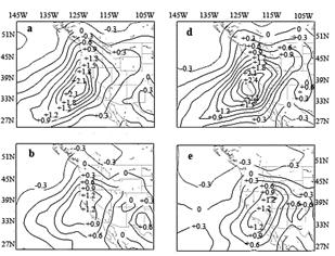
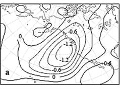
Pattern recognition remains an important component of predicting extreme rainfall events in the mountains along the Pacific coast of North America. The 500-hPa geopotental height and associated anomaly pattern is very similar for all heavy rainfall events with the primary difference being associated with the location of negative anomaly associated with the trough and the positive anomaly to the southeast. Note how similar the anomaly pattern associated with the heavy precipitation events in the Pacific Northwest (below right) to the pattern associated with heavy events in northern California (below right) at the beginning of the period of heavy precipitation. These similarities suggest that once a forecaster is able to recognize the ingredients associated with heavy rainfall in one place along the west coast, he or she should be able to translate that knowledge to enable them to identify possible extreme events in other places along the west coast.

Composite mean 500-hPa departure from normal (positive departures are solid, negative departures are dashed, contour interval=3 dam). Shaded areas are the 95% and 99% probably that the composite belongs to a distinct population from climatology.

Pacific Northwest composite

Northern California composite

From Lackmann and Gyakum 1999

Composite mean 500-hPa normalized departures from normal. Unit is 0.3 standard deviations. Negative values are below normal heights, positive are above normal heights. From Junker et al. 2007.

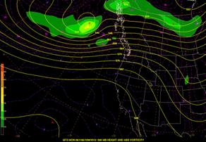
Now we’ll attempt to apply pattern typing and the use of normalized anomalies to forecast a rainfall event over the Pacific Northwest. The first step is to compare the forecast geopotential height field to the composite for heavy events over that area. Note the similarities between the GFS forecast 500-hPa geopotential height field to the composite (below). Both exhibit a fairly strong trough in the height field over the Gulf of Alaska and distinct ridging over California.

582

570

558

546

534

Composite mean 500-hPa height (solid) and sea level pressure (dahsed , every 4 hPa) at the beginning of the period of heavy precipitation over the Pacific Northwest.

12-hr GFS forecast of 500-hPa geopotential height and vorticity valid 1200 UTC 6 Nov. 2006

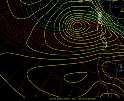
12-hr GFS forecast mslp and 100-500-hPa thickness (dashed) valid 1200 UTC 6 Nov. 2006

Also note the basic look of the forecast mslp pattern with both the surface low position in the Gulf of Alaska and the ridge axis extended from California west-southwest well into the Pacific and compare it to the composite (dashed line, above left). The axis of the area of strongest surface pressure gradient is also similar. However, there is a notable difference, the gradient is much stronger in the forecast than in the Lackmann et al. composite.

Composite mean standardized 500-hPa departure from normal anomalies at the beginning of the period of heavy rainfall, a) for 4 inch or greater events and b) for 2-4 inch events; at the end of the period, c) for 4 inch or greater events, and d) for 2-4 inch events. (from Junker et al. 2007).

Table of contents